Flow Regimes are the behavior of the fluid while flowing in a well. The most common regimes are laminar, turbulent, and transitional. Unfortunately, it is impossible to define each type in the well clearly. For example, mudflow may be predominantly laminar, although the flow near the pipe waIls during pipe rotation may be turbulent.
Laminar Flow.
The most common annular flow regime is laminar. It exists from meager pump rates to the rate at which turbulence begins. Characteristics of laminar flow proper to the drilling engineer are low friction pressures and minimum hole erosion.
Lamina Flow Description
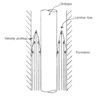
Laminar flow can be described as individual layers, or laminae, moving through the pipe or annulus. The center layers usually move at rates more significant than the layers near the wellbore or pipe. The flow profile describes the variations in layer velocities. The shear-resistant capabilities of the mud control these variations. A high yield point (check also Yield Point In Drilling Mud) for the mud tends to make the layers
move at more uniform rates.
Laminar Flow Associated Problems And Solution
Problem
Cuttings removal is more difficult with laminar flow. The cuttings move outward from the higher-velocity layers to the more compliant areas. These outer layers have very low velocities and may not be effective in removing the cuttings.
Solution
- By increasing the yield point, which decreases layer velocity variations.
- Pumping a 10-20 bbls high-viscosity pill to “sweep”the annulus of cuttings.
Turbulent Flow.
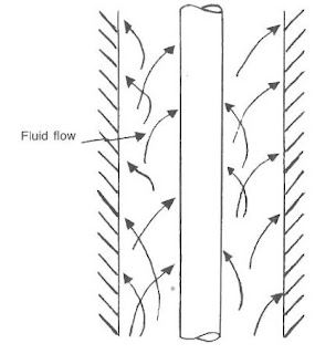
Turbulence occurs when increased velocities between the layers create shear strengths exceeding the ability of the mud to remain in laminar flow. The layered structure becomes chaotic and turbulent.
Turbulence occurs commonly in the drill string and occasionally around the drill collars.
Turbulent Flow Associated Problems
Much published literature suggests that annular turbulent flow increases hole erosion problems. The flow stream is continuously swirling into the walls. In addition, the velocity at the walls is significantly greater than the wall layer in laminar flow. Many industry personnel believes that turbulent flow and the formation type are the controlling parameters for erosion.
Transitional Flow.
Unfortunately, estimating the flow rate at which turbulence will occur is often difficult. In addition, turbulence may occur in various stages. Describing this “gray” area as a transitional stage is convenient.
Flow Regimes Turbulence Criteria.
Several standard methods can be used to establish turbulence criteria. The most common approach is the Reynolds number. Others include:
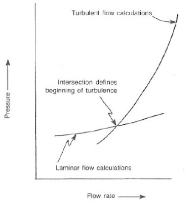
1) Intersection of the flow rate vs. pressure loss calculations for laminar and turbulent flow.
2) Calculation of a z-value.
Reynolds published a paper (1883) that reported experiments dealing with flow in pipes. He injected a thin filament of dye into a moving stream of liquid flowing in a glass pipe. He found that if the numerical value of a group of variables was less than 2,100, the dye filament remained small. The
filament rapidly dispersed in “eddies” if the value of the group was more significant than 2,100.
Turbulence occurs when the ratio of the liquid’s momentum to the liquid’s viscosity ability to dampen permeations exceeds some empirically determined value. The momentum force of the liquid is its velocity times its density. The viscous ability of the liquid to damp out permeations is the internal resistance against change and the effects of the walls of the borehole.
Newtonian Fluids
For the simple case of a Newtonian, nonelastic liquid flowing in a pipe, the dampening effect is the quotient of the viscosity and the diameter of the wellbore:
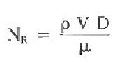
Where:
NR = Reynolds number
ρ = density
D = diameter
μ = viscosity
Non-Newtonian Fluids
Defining a single Reynolds number becomes difficult since drilling muds are non-Newtonian and contain some degree of elasticity. The Reynolds number for the flow of a non-Newtonian liquid in a pipe will be as follows:
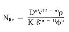
Where:
NRc = effective Reynolds number
n = flow behavior index
k = consistency index
The terms n and K relate to the Power Law mud model, which will be discussed in following sections.
- A simpler equation used in the literature to predict the Reynolds number at the upper limit of laminar flow is as follows:
NRc= 3,470 – 1,370 n
- The relation for the Reynold~ number between the transition and turbulent flow regimes :
NRc= 4,270 – 1,370 n
It is evident from above Eqs. that the Reynolds number is sliding, with its dependency on the flow behavior index.
The position of the intersection between the laminar and turbulent flow pressure losses depends on the equations being used see below figure., The Reed slide rule or. The Hughes tables can make errors if the mud is non-Newtonian at the applicable shear rate. Using well-known equations available in the literature and a Newtonian fluid, the laminar-turbulent pressure lines intersect at a point equivalent to a Reynolds number of approximately 1,900, or 10% below the 2,100 value. The point of intersection for non-Newtonian fluids maybe 30% below the actual transition.
Ryan and Johnson developed the z-value method based on experimental data from several sources and experimentally verified by others. The z-value is calculated from below Eq.:
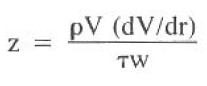
Laminar flow is assumed, and the z-value is calculated and plotted vs. the radius. If the value exceeds 808, the assumption of laminar flow is incorrect, and turbulence occurs. Calculating the z-value is complex and time-consuming
Flow Regimes Critical Velocity.
Critical velocity defines the sit-angle velocity at which the flow regime changes from laminar to turbulent. This variable from above Eq. is the most important since all other members are considered constant in a typical operation. Since no single Reynolds number defines the transitional zone, a range of critical velocities may be necessary to determine the flow regime.
A critical velocity (Vc) and an actual velocity (Va) are calculated in practical applications.
- If Va < Vc, the flow is laminar.
- If Vc < Va, the flow is turbulent.
- If Va = Vc, calculations are made with both flow regimes and the larger pressure losses are used.
Drilling Mud Flow Regimes (Mathematical) Models
A mathematical model is used to:
- Describe the fluid behavior under dynamic conditions.
- Calculate friction pressures
- Calculate swab and surge pressures
- Calculate slip velocities of cuttings in fluids.
The models most commonly used in the drilling industry are:
- Newtonian Model.
- Bingham Plastic Model.
- Power Law Model.
Shear Stress & Shear Rate
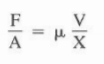
Terms used in mud models are shear stress and shear rate. They can be described by considering two plates separated by a specified distance with a fluid. If a force is applied to the upper plate while the lower plate is stationary, a velocity will be reached and will be a function of the force, the distance between the plates, the area of exposure, and the fluid viscosity:
| Relation Between shear Stress and Shear Rate |
Where:
- F = force applied to the plate
- A = contact area
- V = plate velocity
- X = plate spacing
- μ = fluid viscosity
- F/A is termed the shear stress (?)
- V/X is shear rate (ɣ):

Newtonian Model
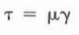
In drilling operations, the shear stress and shear rate are analogous to mud pump pressure and rate, respectively—newtonian Fluids. The model used initially to describe drilling mud was the Newtonian model.

It stated that pump pressure (shear stress) would increase proportionally to the shear rate, as seen in the below figure. If a constant of proportionality is applied to represent fluid viscosity, the above equation will become as follows:
Where:
μ = fluid viscosity
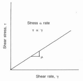
| Newtonian Model |
Unfortunately, a single viscosity term usually cannot describe drilling mud. They require two or more points for an accurate representation of behavior. As a result, the Newtonian model generally is not used in hydraulics plans.
Bingham Plastic Model
The Bingham model was developed to describe drilling muds in use more effectively. Bingham theorized that some amount of stress would be required to overcome the mud’s gel structure before it would initiate a movement as per the below figure:
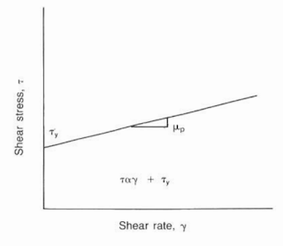
Which can be described by this equation:
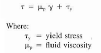
In practical terms, the equation states that a particular pressure would be applied to the mud to initiate movement. Flowing mud pressures would be a function of the initial yield pressure and the fluid viscosity. Shear rates usually are taken at 300- and 600 rpm on the viscometer.
The fluid viscosity (μp)and the yield stress (?y)are calculated as follows:
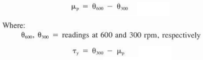
Plastic Viscosity
The fluid viscosity then will be termed plastic viscosity (PV) due to the plastic nature of the fluid and is measured in centipoise (cp). The plastic viscosity is affected by the size, shape, and concentration of particles in the mud system. As mud solids increase, the plastic viscosity increases. The plastic viscosity is a mud property that is not affected by most chemical thinners and can be controlled only by altering the state or number of solids.
Yield Stress
The yield stress, ?y, is given the name of the yield point and is measured in Ib/100 ft^2. It is a function of the interparticle attraction of the solids in the mud. Chemical thinners, dispersants, and viscosifiers control the yield point.
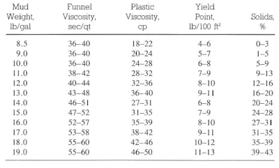
Common Mud Properties
The below tables illustrate common mud properties for gel-based, Oil Based Mud, and invert oil emulsions. These properties were obtained from various mud companies and should be used only as a guide.
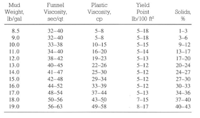
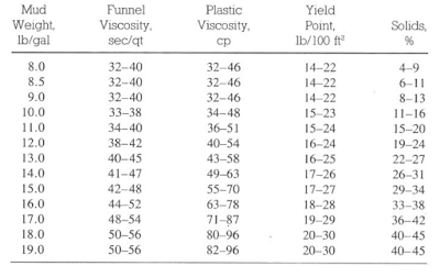
It is difficult to justify using PV and YP terms to oil muds because emulsified water treats a solid particle. Oil Based Mud Figures can be used to describe the weaknesses of the Bingham model. A problem with any model used in drilling operations is its dependence on using two points to define a line that should be known, intuitively, to be nonlinear.
The 300- and 600-rpm shear rates are generally greater than annulus shear rates, resulting in calculated shear stresses greater than the actual values. Although the Bingham model is commonly accepted in practice, a model such as the Power Law would be more descriptive, particularly when the fluid is in turbulence.
Power Law Model
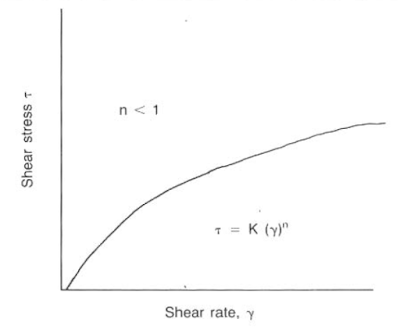
The Power Law model is a standard mathematical expression used to describe a nonlinear curve. The equation for drilling fluids is shown in the below Eq.
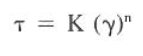
Where:
- K = consistency index
- n = flow behavior index
The flow behavior index describes the degree to which the fluid is non-Newtonian.
The flow behavior and consistency indices are calculated from below Eqs., respectively (is modified slightly for use in Moore’s slip velocity correlation. will be discussed later):
(Above Eq. is modified slightly for use in Moore’s slip velocity correlation. will be discussed later)
This Equation can be described as in below figure
Example For using Power Low Model & Bingham Model:
Use the following viscometer readings to compute PV, YP, n, and K:
θ600 = 64
θ300 = 35
Solution:
- PV = θ600 – θ300 = 64-35 = 29 cp
- YP = θ300 – PV = 35-29 = 6 Ib / 100 ft^2
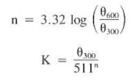
- n = 3.32 x Log ( θ600 / θ300 ) = 3.32 x Log ( 64 / 35) = 0.870
- K = θ300 / 511^ n = 35 / 511 ^ 0.870 = 0.154