Pumping a drilling fluid requires overcoming frictional drag forces from fluid layers and solids particles. In this article, we will explain the pressure loss calculation steps in the drill string. The pump pressure (Pp) can be described as the summation of the frictional forces in the circulation system:
PP = PDS + PB + PA
Where:
- PP: pump pressure, psi
- PDS: drill string friction pressure, psi
- PB: drilling bit pressure drop, psi
- PA : annulus pressure, psi
The pressure drop in the bit results from fluid acceleration and not solely friction forces. As a result, it will be discussed in a separate section.
Equations to determine drill string or annulus pressure loss vary according to the flow regimes, such as laminar and turbulent. In addition, Bingham Plastic and Power Law models differ in form. Since these models are frequently used in drilling applications, they will be presented in the following sections. Newtonian-based equations will not be presented.
Surface Lines Pressure Loss (Friction Pressures).
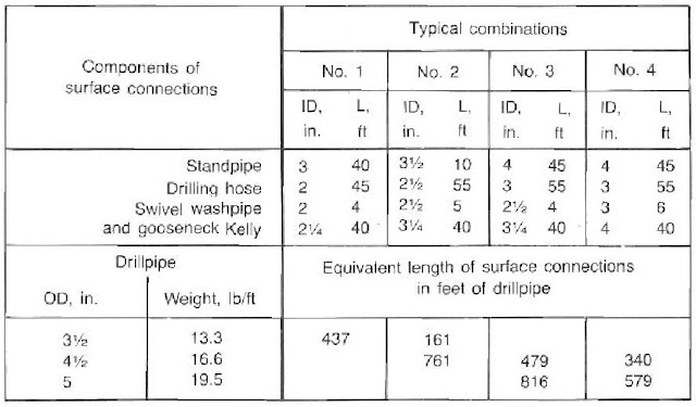
Calculating the pressure drop in surface equipment such as the standpipe and drilling kelly is usually accomplished by equating it to an equivalent length of drill pipe. The surface equipment is separated into four groups (below Fig.) to determine an equivalent length. For example, if a rig has group three surface equipment and 4Y2-in. The drill pipe was used; an additional 479 ft would calculate pressure losses in the surface equipment.
Bingham Plastic Friction Pressures
The Bingham Plastic model is used primarily for pressure loss calculations associated with laminar flow. This restriction is based on its inability to accurately describe shear stresses associated with high shear rates. However, Laminar and turbulent flow calculations will be presented since they are frequently used in the drilling industry.
A – Friction Pressure Calculations in Drill String
1) The velocity of the fluid in the drill string is described as follows:
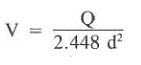
Where:
- V = fluid velocity, ft/sec
- Q = flow rate, gal/min
- d = pipe diameter, in.
2) The critical velocity (Vc) for laminar and turbulence determination is computed below Eq.:
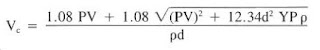
Where:
- Vc = critical velocity, ft/sec
- PV = plastic velocity, cp
- YP = yield point, Ib/l 00 fe (check also Yield Point In Drilling Mud Formula)
- p = mud weight, Ib/gal
3) Drill string pressure loss (Friction pressures) for laminar flow can be calculated as follows:

Where:
- L = section length, ft
4) Drill string pressure loss (Friction pressures) for turbulent flow is calculated according to below Eq.:

B – Friction Pressure Calculations in The Annulus
In the annulus, the same series of operations is performed but with slightly different equations to account for the hole geometry:
1) The velocity of the fluid in the annulus is described as follows:
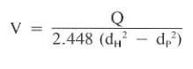
Where:
- dH = casing or hole 10, in.
- dp = pipe or collar 00, in.
2) The critical velocity (Vc) for laminar and turbulence determination is computed below Eq.:
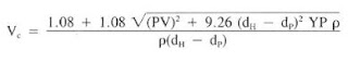
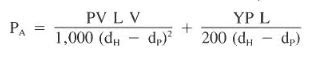
3) Annulus pressure loss (Friction pressures) for laminar flow can be calculated as follows:
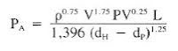
4) Annulus pressure loss (Friction pressures) for turbulent flow is calculated according to below Eq.:
Example For Using Bingham Model In Friction Pressure Calculations
Use the results from the Last Example and the following data to calculate friction pressures for 100 and 200 gpm flow rates. Use the Bingham model.
- pipe ID = 3.5 in.;
- mud weight = 12.9Ib/gal;
- PV = 29 cp;
- YP = 6 Ib/100 ft;
- length = 10,000ft
Solution:
1. Calculate the velocities for flow rates of 100 and 200 gal/min:

V = 100 / 2.448 x 3.5^2 = 3.33 ft/sec (at 100 gal/min)
V = 200 / 2.448 x 3.5^2 = 6.66 ft/sec (at 200 gal/min)
2. Determine the critical velocity at which laminar flow will convert to turbulent flow:
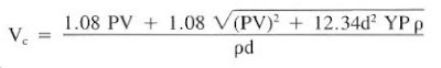
Vc = (1.08 x 29 + 1.08 x ( 29^2 + 12.34 x 3.5^2 x 6 x 12.9)^(1/2)) / (12.9 x 3.5 ) = 3.37 ft/s
3. Calculating Friction Pressure For 100 gal/min
For the 100 gal/min flow rate, the actual velocity (Va) is slightly less than the critical velocity (Vc)of 3.37 ft/sec. Use the laminar flow equation. (Note that the difference between Va and Vc is slight. Therefore, it might be advisable in some cases to consider calculating pressure losses for laminar and turbulent flow and use the greater value.)
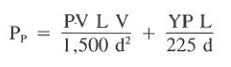
Pds = (29 x 10000 x 3.33) / (1500 x 3.5^2) + (6 x 10000) / ( 225 x 3.5) = 52.5+76.1= 128.6 psi
4. Calculating Friction Pressure For 200 gal/min
At a flow rate of 200 gal/min, the actual 6.66 ft/sec velocity is significantly greater than the critical velocity of 3.37 ft/sec. Therefore, use the turbulent flow equation:
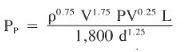
Pds = ( 12.9 ^ 0.75 x 6.66^1.75 x 29^ 0.25 x 10000) / ( 1800 x 3.5 ^ 1.25) = 505.7 psi
The Difference Between Friction Pressure Calculations In Both Laminar & Turbulent Flow
The laminar and turbulence equations can be used to illustrate the fundamental difference between these two flow systems. In the laminar equations, a value for the yield point (YP) is a significant part of the pressure loss, mainly when it is observed that the PV value is divided by a squared diameter. The
turbulent flow equations do not contain a YP term. The yield point is one of the forces creating the inter-particle attractions, causing the mud to move in laminar. When the shear force exceeds the yield stress, turbulence begins, and the yield point is not a factor after that.
Power Law
Power Law calculations follow the same sequence as the Bingham model. Actual and critical velocities are compared to determine the flow regime before calculating the pressure loss.
- If Va and Vc differ significantly, choose the appropriate flow equation.
- When Va = Vc make both pressure loss computations and choose the larger.
A word of caution must be given relative to Bingham and Power Law equations. Many forms of these computations exist in the industry, with slightly differing units. Velocity can be expressed in ft/sec or ft/min, which obviously would make a significant error in the calculations, particularly when V is in exponent form.
The Power Law model demands additional attention because several methods exist for computing the basic parameters of n and K. This is not the case for the Bingham model because only one accepted method is used for PV and YP calculations. The equations presented in this text are those of Moore et al.
A – Pressure Loss Calculations in Drill String
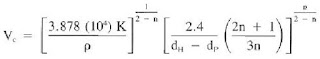
For computation simplicity, NR = 3,000 is assumed for turbulence criteria. Basic assumptions for friction factor correlations result in the critical velocity equation:

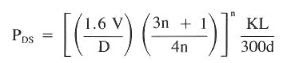
Calculating pressure loss (friction pressures) in the drill string using the Power Law equations for laminar flow:
Calculating Pressure loss (friction pressures) in the drill string using the Power Law equations for turbulent flow:
B – Pressure Loss Calculations in The Annulus
Calculating critical velocity equation
Calculating pressure loss (friction pressures) in the annulus using the Power Law equations for laminar flow:
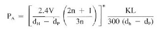
Calculating Pressure loss (friction pressures) in the annulus using the Power Law equations for turbulent flow:
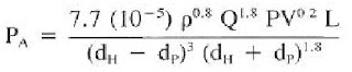
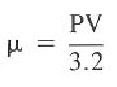
Note that the above equation uses the PV term, a Bingham model value. Since it is value to relate viscosity to a turbulent flow, a common practice uses μ related to PV, as shown below:
Example Of Using Power Law
Refer to the above Examples and compute the friction pressures for the system in the above Example. Use the Power Law model and a flow rate of 125 gal/min. If Va is nearly equal to Vc, compute the pressure drop for laminar and turbulent flow and choose the more significant value.
Solution:
l) Referring to the above Examples, the data to be used are:
- n = 0.870
- K = 0.154
- pipe ID = 3.5 in
- mud weight = 12.9 Ib/gal
- length = 10,000 ft
2) Determine the actual velocity at 125 gal/min:

Va = 125 / (2.448 x 3.5^2) = 250 ft / min
3) Use the Below Equation to compute the critical velocity, Vc:
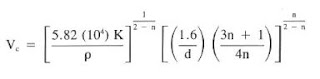
Vc = (6.947 x 10^2) ^ 0.884 x (0.474 ^ 0.7699) = 325 x 0.563 = 183 ft / min = 3.05 ft / sec
For purposes of illustration in this example, assume that Va of 250 ft/min nearly equal Vc of 183 ft/min.
4. Calculating Laminar flow pressure losses (friction pressure)

PDS = ( ( 1.6 x 250 / 3.5) x ( 3 x 0.870 +1) / (4 x 0.870)) ^ 0.870 x ((0.154 x 10000) / (300 x 3.5))
= 95.4 psi
5) Calculating Turbulent flow pressure losses (friction pressure)
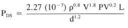
PDS = (2.27 x 10 ^ -7 x 12.9 ^ 0.8 x 250 ^ 1.8 X 10000) / 3.5 ^1.2 = 158.6 psi
6) Assuming the pressure loss is greater Since 158.6 psi> 93.4 psi.
7) Some groups within the industry bypass Step 3 altogether and compute the pressure drops from both laminar and turbulent equations
So great