A spinner log records the response of a rotating impeller to fluid moving past it. Turning that response into an interval contribution requires more than reading revolutions per second from a track. The interpretation must account for tool motion, calibration, the velocity distribution across the flow passage and, where several phases coexist, how those phases occupy and move through the well. [1, pp. 4-3–4-8]
This article follows that conversion from signed relative motion to a defensible flow profile in a completed oil well. It focuses on the interpretation behind the curve rather than surveying every production-logging sensor. The original examples use invented inputs, and none supplies recommended logging speeds, a minimum detectable field rate or an operating program. The workover operations article places flow diagnosis within wider intervention objectives.
What does a spinner log actually measure?
The impeller responds to fluid motion relative to the instrument. The recorded rotation can be related to velocity through a response model, but the relationship also depends on the spinner and the fluid. Density, viscosity and mechanical friction matter. A rotation value is therefore an instrument response, not an oil rate, water rate or direct measure of the contribution from the nearest perforation. [1, pp. 4-5 and 4-7–4-8]
The source describes continuous, fullbore and diverter flowmeters. They interact with different portions of the flow passage and do not provide identical sampling. A larger spinner can sample more of the cross section; a diverter changes the route through which fluid reaches the measurement section. These functional distinctions do not justify transferring one device’s calibration or historical performance figures to another. [1, pp. 4-5–4-7]
Depth and time also belong with the response. A change must be assigned to the correct completion interval, while separate passes need sufficiently comparable well conditions for their relationship to be meaningful. Schlumberger describes simultaneous production measurements, depth-correlation sensors and interpretation under stable flowing or injecting conditions. The measurement record should preserve that context rather than presenting an isolated spinner curve. [1, pp. 4-1–4-2]

Choose the sign convention before comparing motion
For the examples here, upward axial velocity is positive for both the fluid and tool. The fluid velocity relative to the spinner is then:
urelative = ufluid − utool
This is a stated coordinate convention, not a universal logging-display convention. The reference uses its own direction definitions in its response equations. What matters is that the tool-speed record, rotation direction and interpretation use consistent signs. A sign taken from one display should not be combined silently with a different definition from another. [1, pp. 4-7–4-8]
Suppose fluid moves upward at an invented +0.30 m/s. A tool moving downward at −0.20 m/s experiences +0.50 m/s of relative flow. If it instead moves upward at +0.30 m/s, relative velocity is zero even though fluid is moving upward in the well. At +0.60 m/s tool speed, relative flow is −0.30 m/s: the tool has overtaken the fluid.
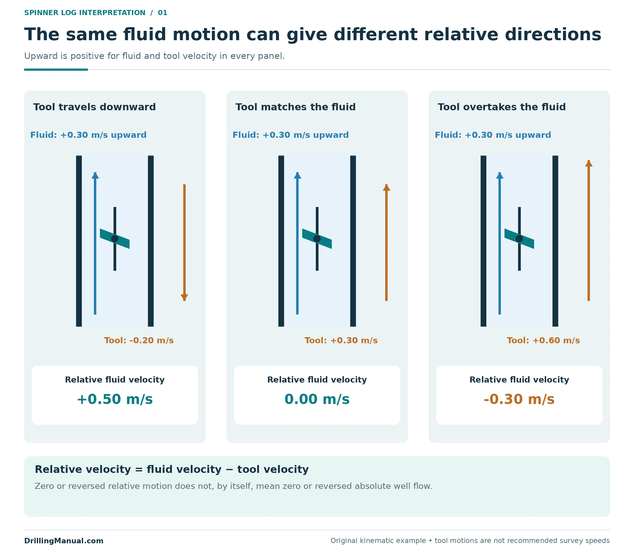
Thus, reversed rotation during a pass does not automatically mean the well fluid reversed its absolute direction. Likewise, a zero rotation observation cannot establish zero well flow without the tool-motion and response context. These are consequences of relative motion, before any further complication from multiphase flow is introduced. [1, pp. 4-5 and 4-7–4-8]
Spinner log thresholds and response branches
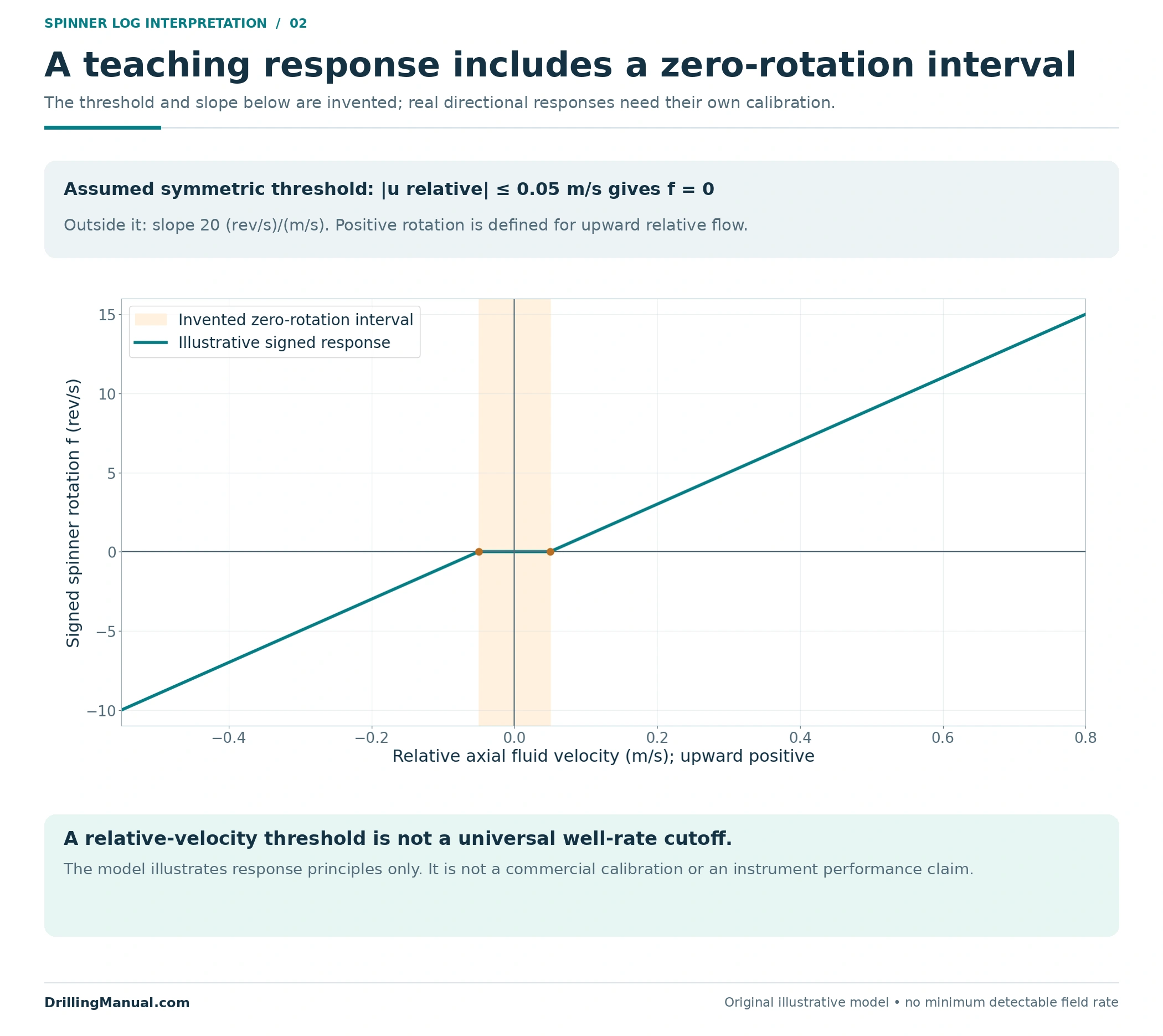
The ideal response line is a useful starting picture, but friction and fluid effects alter the behavior around low relative velocity. The book shows separate response branches and threshold offsets, with approximately straight behavior at higher rotation rates. It also explains that the inferred velocity depends on the response-line intercepts and thresholds. A low-response region should not be treated as a universal field-rate boundary. [1, pp. 4-7–4-8]
For a transparent teaching model, assume the spinner does not rotate when the magnitude of relative velocity is at most 0.05 m/s. Outside that interval, assume a slope of 20 revolutions per second for each m/s above the threshold. Define positive rotation to correspond to upward relative flow. Both thresholds and both slopes are deliberately symmetric in this invented model; real calibration need not have that symmetry.
For |urelative| ≤ 0.05 m/s: f = 0. Otherwise: f = 20 × sign(urelative) × (|urelative| − 0.05).
The factor 20 carries units of (rev/s)/(m/s), and f is signed rotation in rev/s. This equation is original illustrative arithmetic informed by the source’s response principles. It is not a fit to a commercial tool and must not be used to select a survey speed or a minimum well rate. [1, pp. 4-7–4-8]
A spinner log threshold is expressed here in relative velocity, not in barrels or cubic metres per day. Converting a velocity to a volume rate requires a flow area and an appropriate velocity interpretation. The same numerical velocity in two different passages does not imply the same rate. That distinction is one reason a threshold quoted without geometry and fluid context is incomplete. [1, pp. 4-3 and 4-7–4-8]
An illustrative multipass spinner log calibration
Hold the invented fluid velocity at +0.30 m/s and apply the teaching response model to several tool velocities. Each row represents the same assumed fluid state with a different tool motion. This separates the effect of moving the instrument from a change in the well itself.
| Tool velocity, m/s | Relative fluid velocity, m/s | Signed rotation, rev/s |
|---|---|---|
| −0.40 | +0.70 | +13 |
| −0.20 | +0.50 | +9 |
| 0.00 | +0.30 | +5 |
| +0.20 | +0.10 | +1 |
| +0.40 | −0.10 | −1 |
| +0.60 | −0.30 | −5 |
Plotting rotation against tool velocity exposes the two response branches. Their extrapolated zero-rotation intercepts occur at +0.25 and +0.35 m/s. In this particular symmetric model, their midpoint is +0.30 m/s, the assumed fluid velocity. That midpoint rule follows from the stated symmetry; it is not a general substitute for interpreting actual directional thresholds and calibration behavior.
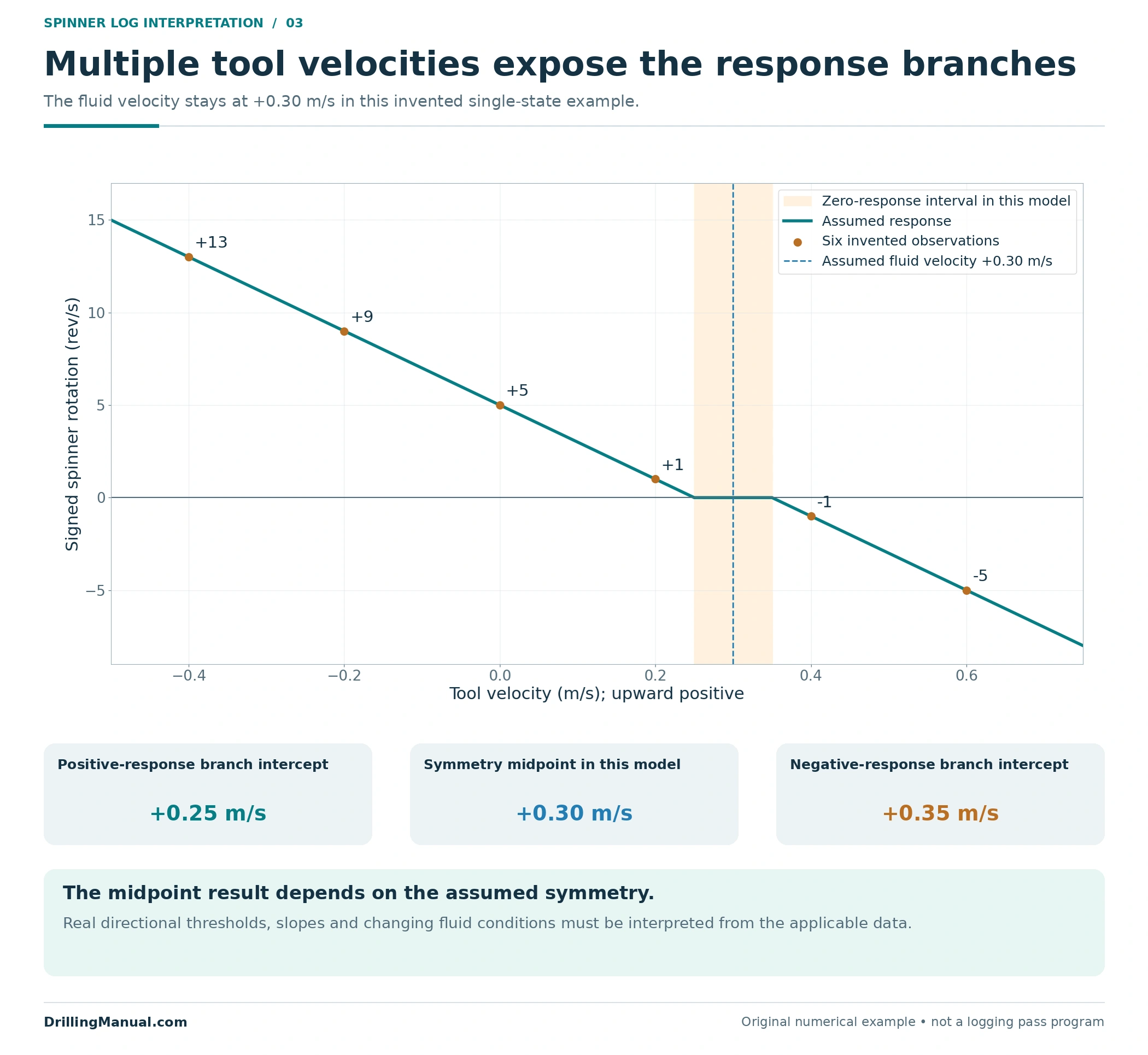
The purpose of multiple passes is to constrain the relationship between rotation and tool motion within the relevant fluid environment. The source describes crossplots for selected intervals of consistent spinner response, rather than applying one unexplained rotation-to-rate conversion throughout the well. It also qualifies percentage allocation when density, viscosity or velocity profiles change. [1, pp. 4-7–4-9]
A credible calibration comparison must still explain inconsistent passes. If the fluid state changed between them, a single response line may combine different conditions. More plotted points do not resolve that problem automatically. Pressure and other contemporaneous channels help establish what state the measurements describe. [1, pp. 4-1–4-2 and 4-7–4-9]
Percentage contributions do not always avoid the calibration problem. The source’s simpler single-phase allocation assumes consistent density, viscosity and velocity profile across the interpreted interval. If those assumptions fail, relative deflections can cease to represent comparable flow changes. A spinner log report should state why percentage allocation is supported, rather than presenting percentages as inherently more reliable than an absolute rate. [1, p. 4-7]
From sampled velocity to a volume rate
Even after tool motion has been accounted for, the sampled fluid velocity need not equal the average velocity across the entire passage. In single-phase flow, fluid near the center can move faster than fluid near the wall. The source discusses different velocity profiles and a correction from measured to average velocity. A correction belongs to the relevant conditions; no single numerical factor is adopted here. [1, pp. 4-2–4-3 and 4-8]
For a defined single-phase flow area A, the volume rate is Q = A × ū, where ū is the appropriate cross-sectional average velocity. This step requires both an area and a representative velocity. Applying the pipe area to an uncorrected local reading can produce a plausible-looking rate without establishing that it describes the whole passage. [1, p. 4-3]
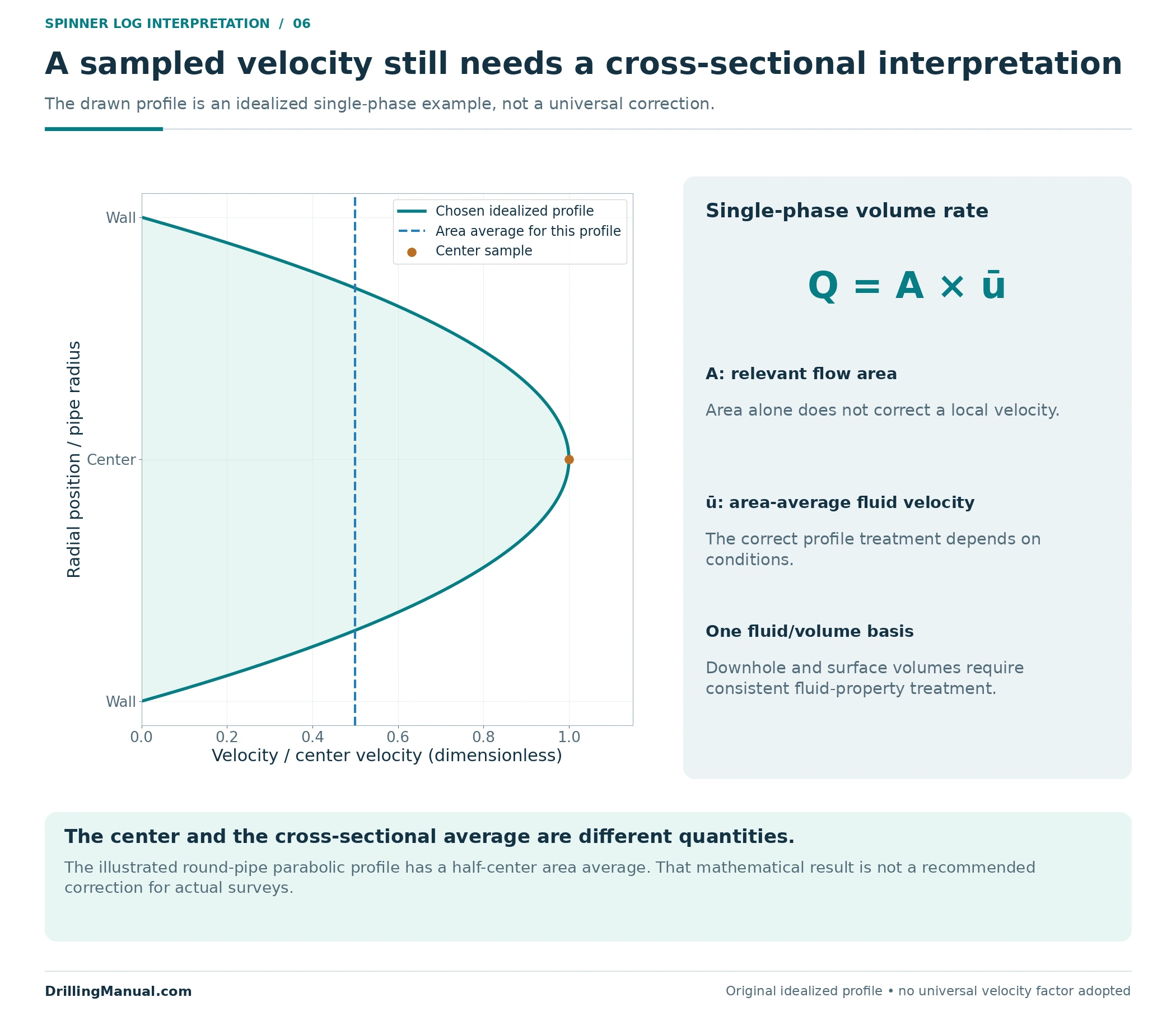
Downhole and surface volumes also require a common fluid-property basis before comparison. Pressure and temperature affect fluid densities, viscosity and phase behavior. The book emphasizes downhole conditions and fluid-specific PVT information in production-log interpretation. A numerical match between quantities expressed on different bases is not a valid reconciliation. [1, pp. 4-4–4-5]

Build a spinner log flow profile from interpreted rates
Consider a separate hypothetical vertical well with three open intervals: C at the bottom, B in the middle and A at the top. Assume steady single-phase flow, a valid calibration and area/velocity interpretation, one common downhole volume basis, and no unmeasured bypass or storage change. The rates below are already interpreted cumulative rates. They are not the raw rotations from the preceding calibration example.
| Measurement section | Cumulative upward rate, m³/day |
|---|---|
| Below C | 0 |
| Between C and B | 160 |
| Between B and A | 140 |
| Above A | 200 |
Under those assumptions, an interval’s net contribution is the rate just above it minus the rate just below it. C adds 160 m³/day. B has a net contribution of 140 − 160 = −20 m³/day, meaning it receives fluid in this constructed case. A adds 200 − 140 = 60 m³/day. The net total is 160 − 20 + 60 = 200 m³/day.
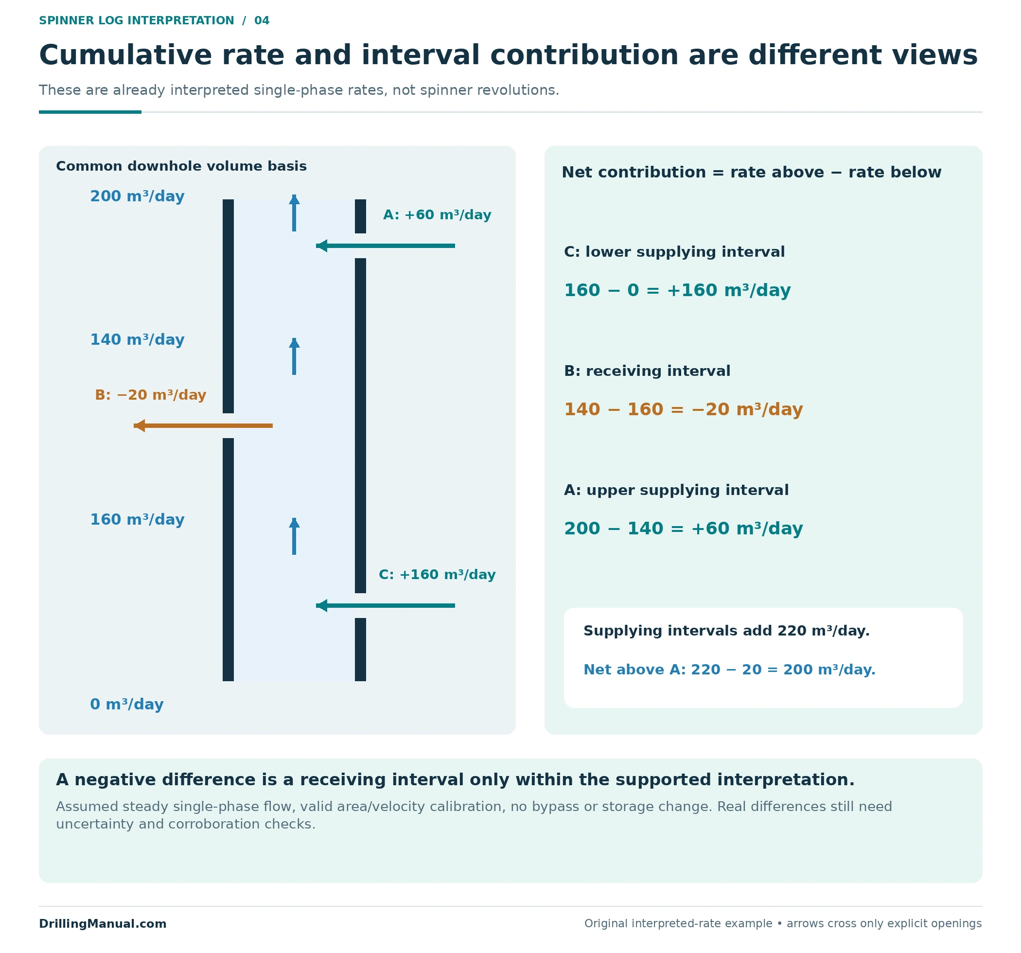
The negative increment is deliberate. It shows why cumulative upward flow need not increase across every open interval. The source recognizes thief intervals and their effect on interpretation. In actual data, however, a small calculated decrease needs comparison with repeatability, calibration quality and supporting measurements before it is assigned to a receiving zone. The arithmetic alone cannot validate the interpretation. [1, pp. 4-2 and 4-7–4-9]
In this invented spinner log interpretation, the two supplying intervals together add 220 m³/day, while 20 m³/day leaves through B. The net rate above all intervals is therefore 200 m³/day. Reporting only that final number would conceal the receiving interval. Equally, summing only the positive contributions would overstate the net upward rate. Both cumulative and incremental views belong with the stated common volume basis.
An inventory of perforated intervals establishes where connections were intended; it does not establish their current contributions. A multiple-zone completion must also be interpreted using its actual communicating paths. A total-rate change cannot be assigned to the nearest formation if another route can explain it. [1, pp. 4-1–4-2]
Why multiphase and deviated flow change the interpretation
In multiphase flow, different fluids can travel at different velocities. Holdup describes their local volume occupancy; it does not by itself give their shares of the flowing rate. A spinner log therefore needs suitable phase-sensitive information and a flow interpretation before its response is divided into oil, water and gas contributions. [1, pp. 4-4–4-5]
Deviation can make the sampling problem more pronounced. Gravity can separate fluids across the passage, and the source describes circumstances in which heavier liquid moves down locally while lighter fluid continues upward. A spinner encountering that local motion may indicate a direction that does not describe the net movement of all fluid across the section. This is a possible flow pattern, not an inevitable consequence of every deviated well. [1, p. 4-5]
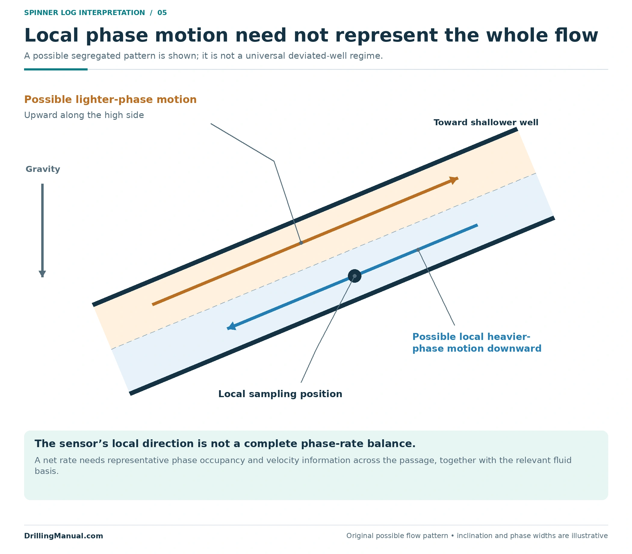
A larger sampling span or a different flowmeter arrangement may address part of the problem, but physical passage through the well is not proof of representative measurement. The book distinguishes conventional, fullbore and diverting devices precisely because their sampling and flow interaction differ. Their suitability must be evaluated against the actual flow regime and measurement objective. [1, pp. 4-5–4-7]
For a water-shutoff decision, the required result is normally more specific than total flow or local water occupancy. The interpretation must identify a supported water contribution and its associated path, while retaining any oil contribution that the proposed isolation could affect. This applies the distinction between flow profiling, phase information and completion diagnosis. [1, pp. 4-1–4-5]
How to read a flat or reversed spinner log
“Flat” can mean constant rotation with depth, or it can mean rotation near zero. Those are different observations. A constant nonzero response may be consistent with unchanged through-flow between entries under stable conditions. Near-zero rotation can instead arise from small relative velocity, including a tool moving with the fluid, or from the response threshold. Neither description should be converted immediately into zero interval contribution. [1, pp. 4-7–4-8]
| Observed behavior | Question before assigning a flow result |
|---|---|
| Near-zero rotation | What was the signed tool velocity, and where is the applicable response threshold? |
| Constant nonzero rotation across a depth interval | Were area, fluid properties, sampling and well conditions sufficiently consistent? |
| Reversed rotation | Did the tool overtake the fluid, or is there evidence of local reverse fluid motion? |
| Different responses on repeat passes | Do the data support one calibration state, or did the well or sampled mixture change? |
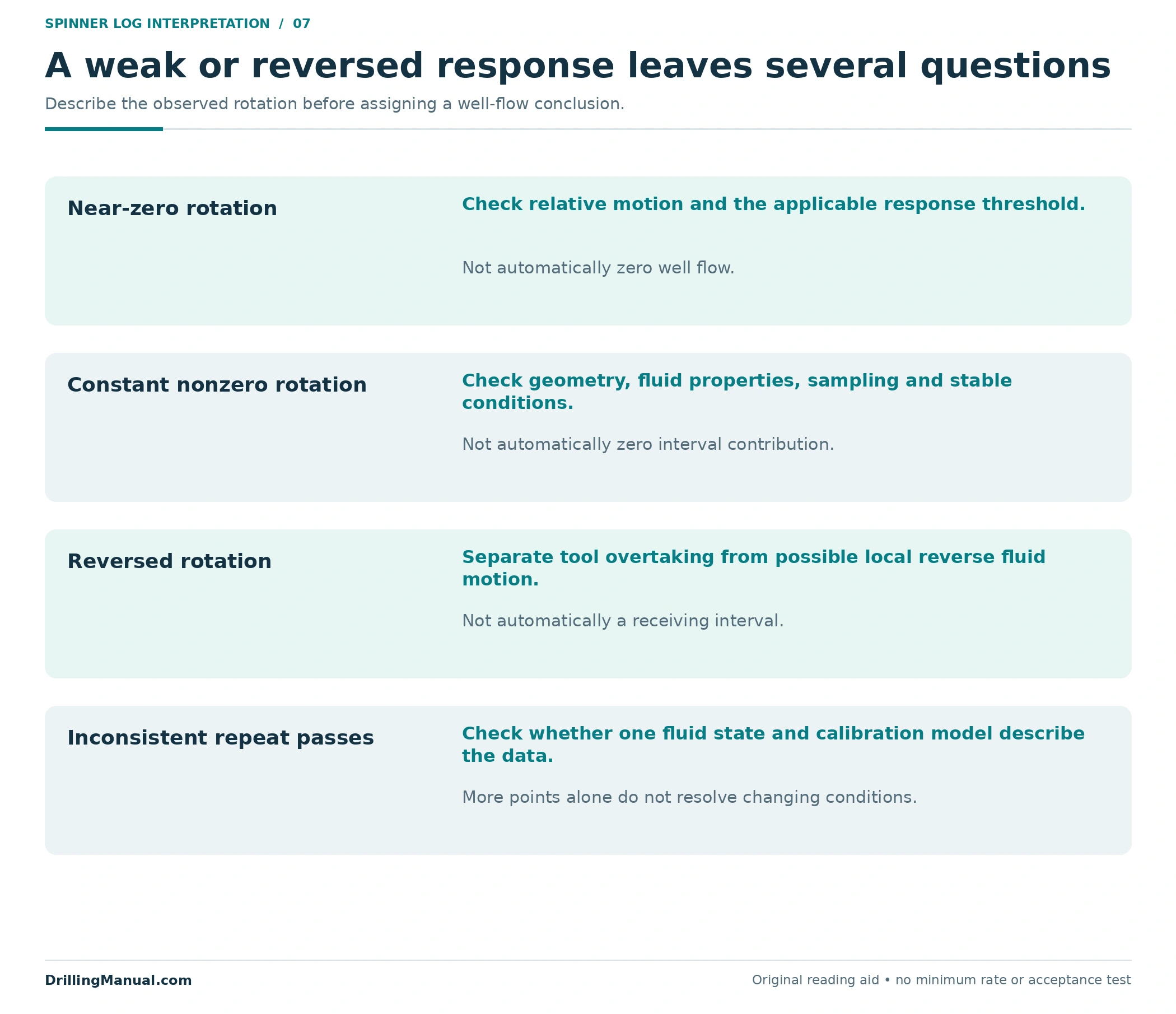
These questions help define the remaining ambiguity. They do not turn every weak response into a successful quantitative survey. Where the measurement cannot support reliable rate allocation, the report should preserve a qualitative finding and identify what remains unresolved rather than manufacture precise phase rates. [1, pp. 4-1–4-8]
Geometry is another reason to distinguish a response change from an inflow change. For the same single-phase volume rate, a larger flow area corresponds to a lower average velocity. Conversely, a restriction can increase average velocity without adding fluid. The spinner log interpretation must therefore relate a depth change to both the completion dimensions and the fluid response before assigning it to a reservoir interval. [1, p. 4-3]
What belongs in the interpretation record?
A useful record connects each final rate to its supporting evidence: depth reference, operating state, signed tool speeds, rotation data, calibration intervals, response model, flow area, velocity-profile treatment and fluid basis. Where several phases are present, it also identifies the phase-sensitive measurements and the assumptions used to resolve their rates. These are review categories derived from the source’s interpretation requirements, not a prescribed survey sequence. [1, pp. 4-1–4-9]
The casing collar locator guide addresses the separate depth-reference problem. Correctly locating a feature does not establish its cause or rate. Preserve the relationship between the completion interval, measurement depth and the final allocation so that a later repair proposal can be checked against the actual evidence. [1, pp. 4-1–4-2]

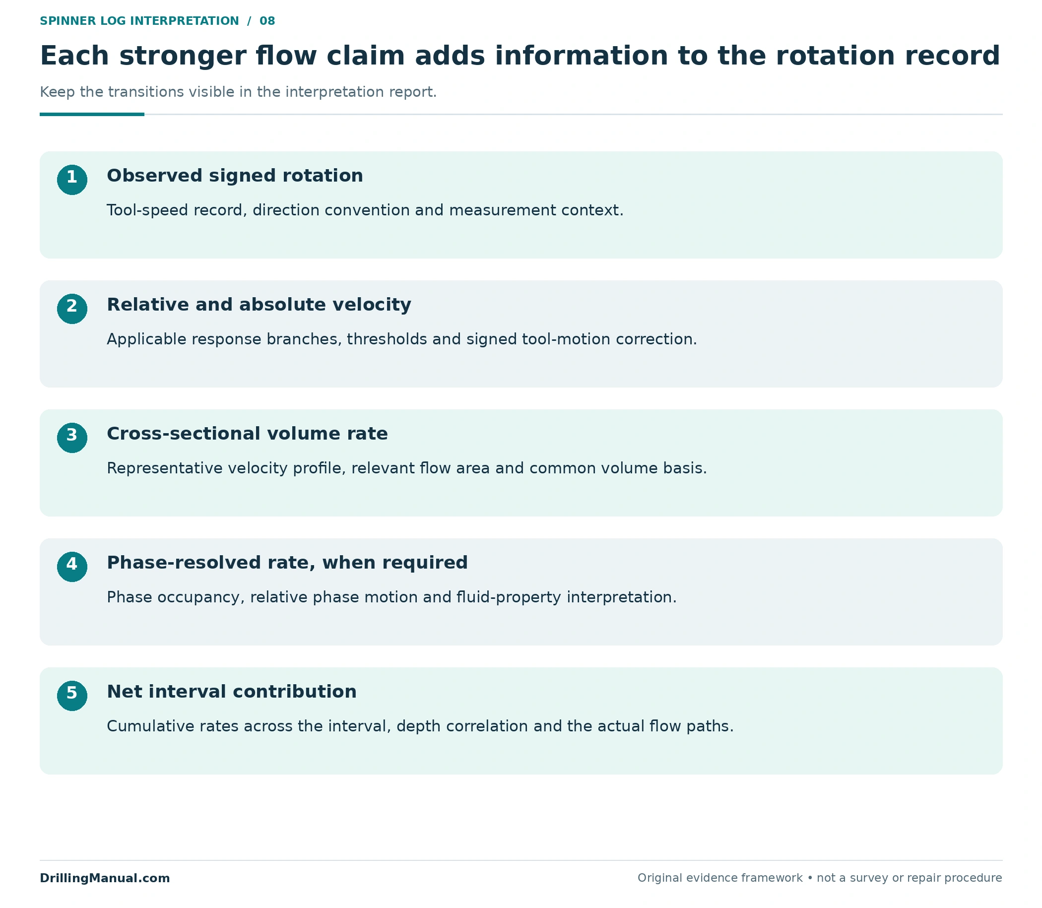
The final spinner log conclusion should distinguish observed rotation, interpreted velocity, cumulative rate and interval contribution. Each transition needs an explanation. If a later survey is used to assess a workover, compare the relevant flow state and rate basis before attributing an altered profile to the intervention itself. [1, pp. 4-1–4-2 and 4-5–4-9]
For a spinner log with an unresolved phase or calibration ambiguity, say which conclusions remain usable. A supported entry location may still help define the next investigation even when an exact phase rate is unavailable. This keeps the evidence useful without making the intervention depend on precision the survey has not established. The level of the claim should follow the available measurement support. [1, pp. 4-1–4-9]
Frequently asked questions
Does zero rotation on a spinner log mean zero flow?
No. Rotation depends on motion relative to the tool and on the response threshold. In the stated velocity convention, fluid and tool moving upward together have zero relative velocity. The interpretation therefore needs tool speed and calibration before a zero response can be connected to a fluid-flow conclusion. [1, pp. 4-5 and 4-7–4-8]
Why compare upward and downward passes?
Changing tool motion provides different relative velocities within the same interpreted interval. The resulting rotation-versus-tool-speed relationship helps constrain response branches and fluid velocity. This comparison is meaningful only with appropriate fluid and well-state context; a universal pass count or logging speed does not follow from the principle. [1, pp. 4-7–4-9]
Can a spinner alone determine the water rate?
Not generally in multiphase flow. The response does not uniquely supply phase occupancy and each phase’s velocity. Holdup, fluid properties and suitable interpretation support are needed to distinguish water movement from oil or gas movement. Downhole volumes also need appropriate conversion before comparison with a surface water rate. [1, pp. 4-4–4-5]
Does reversed rotation prove a thief zone?
No. Tool motion can reverse the relative flow past the impeller without reversing absolute fluid movement. Local counterflow in a segregated mixture is another possible explanation. A receiving interval is a conclusion about the interpreted flow balance across that interval, supported by the full survey context. [1, pp. 4-5 and 4-7–4-8]
Is there one minimum rate for a spinner log?
No universal value is supplied here. The relevant response depends on the selected device, relative velocity, fluid properties and how flow is sampled. Historical source examples describe particular arrangements and test conditions. They should not be promoted into a minimum detectable rate for every oil well. [1, pp. 4-5–4-8]
Does a matching total prove the zonal allocation?
No. An internally consistent sum checks the accounting, not every measurement or model assumption. Depth, calibration, phase interpretation, flow paths and volume basis still need support. A reconciled total can coexist with an incorrect division among intervals, so the detailed interpretation must remain available for review. [1, pp. 4-1–4-9]
Book reference
- Schlumberger. Cased Hole Log Interpretation: Principles/Applications. Copyright 1989; fourth printing, March 1997. Schlumberger Educational Services / Schlumberger Wireline & Testing, SMP-7025. Chapter 4, Completion Evaluation: printed pp. 4-1–4-9 / physical PDF pp. 68–76. The signed response model, multipass numbers, zonal rates, diagrams and review frameworks are original educational examples. They are not reproduced field data, instrument specifications or operating instructions.