The decision to fish or not must be weighed against a need to preserve the wellbore, recover costly equipment, or comply with regulations. Each choice is fraught with its costs, risks, and repercussions. This is why learning how to calculate the economic and optimum fishing time is important.
Before committing to a specific course of action, the operator must consider several factors:
- Fishing costs: daily fee for fishing expertise and daily rental charges for fishing tools and jars,
- Well parameters: proposed total depth, current depth, depth to the top of the fish, and daily drilling rig operating costs including rig personnel rates;
- Lost-in-hole costs: the value of the fish minus the cost of any components covered by tool insurance,
- Fishing timetable: time spent mobilizing fishing tools and personnel, estimated duration of the fishing job, and the probability of success.
Optimum Fishing Time Calculation Formulas
Earlier research has derived equations to determine how long fishing operations can be economically justified. These were based on Gulf of Mexico wells. The work presented here investigates the economics of fishing in the North Sea. The effort was justified by an early BP task force review, which showed that the Gulf of Mexico and the North Sea have significantly different pipe sticking problems.
In the Gulf of Mexico, the most stuck pipe is due to differential sticking. Spotting a diesel-based pill is considered to be the most successful remedy. Mechanical sticking is a significant problem in the North Sea, and the best remedial action needs to be more prominent. Spotting a pill is only one option among many possible options.
In 1984, Keller et al. (1984) introduced the concept of Economic Fishing Time (EFT). They developed an equation to calculate the time the cost of fishing becomes equal to the cost of an immediate well sidetrack. They considered that the probability of successful fishing can be estimated as follows:
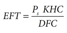
Where:
- EFT = Economic fishing time in days (not optimum).
- Ps = Probability of successful fishing.
- KHC = Known hole costs (Value of fish + cost to re-drill to original depth).
- DFC = Daily fishing cost.
They characterized the fishing times of an EFT using the Weibull distribution, which has the following probability density function (PDF)
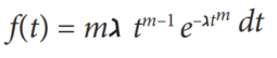
Where:
- t = Time in hours
- = Weibull scale parameter
- m = Weibull shape parameter
We can get the probability of freeing the pipe before time t from the cumulative distribution function (CDF):
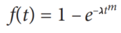
Where f(t) is the time-dependent probability of freeing the stuck pipe. Using f(t) instead of a fixed probability and setting t = EFT, we can rewrite Eq. (1) as:
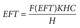
Where:
- EFT = Economic fishing time (not optimum).
- H = Hourly fishing cost
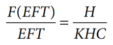
In addition, we can arrange it to give the cost ratio which will be:
Economic Considerations
During any fishing operation, it is important to consider a significant trade-off. Although the actual cost of fishing is usually insignificant in comparison with the cost of the drilling rig and other investments that support the overall drilling operation. In addition, failure to timely remove a fish or junk from the borehole may necessitate sidetracking, which involves drilling around the obstruction or drilling another borehole altogether.
Thus, the economics of the fishing operation and other costs at the well site must be carefully and continuously assessed while the fishing operation is underway. Knowing when to terminate the fishing operation and get on with the primary objective of drilling a well is essential. In such case, Eq. (1) can be rewritten in terms of the number of days (Df) that should be allowed for fishing operation as:
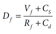
Where:
- Vf = The replacement value of the fish, $
- Rf = The charges per day of the fishing tool and services, $/day
- CS = Estimated cost of the sidetrack or the cost of restarting the well, $
- Cd = The charge per day of the drilling rig (and appropriate support), $/day
Optimum Fishing Time (OFT)
OFT is an economically attractive alternative native to EFT because it attempts to minimize total costs. When fishing operations are started, there are only two possible outcomes: getting free or failing to be free. The costs associated with these outcomes are:
Cost free = Ht EQ.7
Cost fail = Ht + KHC EQ. 8
The probability of getting free is given by Eq. (3). The expected cost (EC) of a stuck pipe incident is, therefore:
EC = Ht F(t) + { 1- F(t)} x { KHC + (H x t)} EQ. 9
That we can simplify to :
EC = Ht+ KHC – KHC F(t) EQ. 10
The gradient equation is given by:
Gradient = F(t) KHC – H EQ. 11
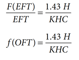
OFT is the point at which the gradient becomes zero, which can be derived from Eq. (11) as:
f (OFT) = H / KHC EQ. 12
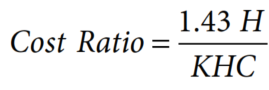
Assuming that the hourly rate for Remedial Operation Time (ROT) is similar to that for fishing, Eqs. (5) and (12) may be rewritten as follows:
In such case, the calculation for the Cost Ratio must be:
If ROT is not considered, the recommended fishing time will be longer than the true the optimum or economic OFT. All the necessary information is now available to complete the new fishing equation. By substituting the terms in Eq. 15), the equation becomes:
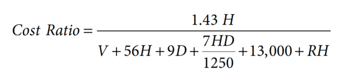
Where:
- v = Value of drillstring below stuck point (US$)
- D = Estimated depth of stuck point (meters)
- H = Hourly rig operating rate (US$)
- R = Time taken to drill original hole below stuck point (hours)